Contents

% maxent_example.m
%
% Example code for the maximum entropy toolkit
% Ori Maoz, July 2016:  orimaoz@gmail.com,


%
% Note: all the "maxent." prefixes before the function calls can be omitted by commenting out the following line:
%import maxent.*

part 1: working with small distributions of neurons (exhaustively)

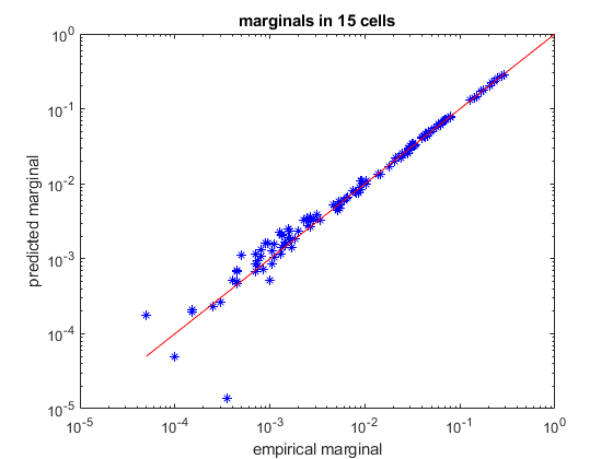
% load spiking data of 15 neurons
load example15

% randomly divide it into a training set and a test set (so we can verify how well we trained)
[ncells,nsamples] = size(spikes15);
idx_train = randperm(nsamples,ceil(nsamples/2));
idx_test = setdiff(1:nsamples,idx_train);
samples_train = spikes15(:,idx_train);
samples_test = spikes15(:,idx_test);

% create a k-pairwise model (pairwise maxent with synchrony constraints)
model = maxent.createModel(ncells,'kising');

% train the model to a threshold of one standard deviation from the error of computing the marginals.
% because the distribution is relatively small (15 dimensions) we can explicitly represent all 2^15 states
% in memory and train the model in an exhaustive fashion.
model = maxent.trainModel(model,samples_train,'threshold',1);

% now check the kullback-leibler divergence between the model predictions and the pattern counts in the test-set
empirical_distribution = maxent.getEmpiricalModel(samples_test);
model_logprobs = maxent.getLogProbability(model,empirical_distribution.words);
test_dkl = maxent.dkl(empirical_distribution.logprobs,model_logprobs);
fprintf('Kullback-Leibler divergence from test set: %f\n',test_dkl);

model_entropy = maxent.getEntropy(model);
fprintf('Model entropy: %.03f   empirical dataset entropy: %.03f\n', model_entropy, empirical_distribution.entropy);

% get the marginals (firing rates and correlations) of the test data and see how they compare to the model predictions
marginals_data = maxent.getEmpiricalMarginals(samples_test,model);
marginals_model = maxent.getMarginals(model);

% plot them on a log scale
figure
loglog(marginals_data,marginals_model,'b*');
hold on;
minval = min([marginals_data(marginals_data>0)]);
plot([minval 1],[minval 1],'-r'); % identity line
xlabel('empirical marginal');
ylabel('predicted marginal');
title(sprintf('marginals in %d cells',ncells));

Training to threshold: 1.000 standard deviations
Maximum MSE: 1.000
converged (marginals match)
Standard deviations from marginals: 0.097 (mean), 0.987 (max) [9]  DKL: 0.102
Kullback-Leibler divergence from test set: 0.098116
Model entropy: 6.464   empirical dataset entropy: 6.384

part 2: working with larger distributions of neurons (MCMC)

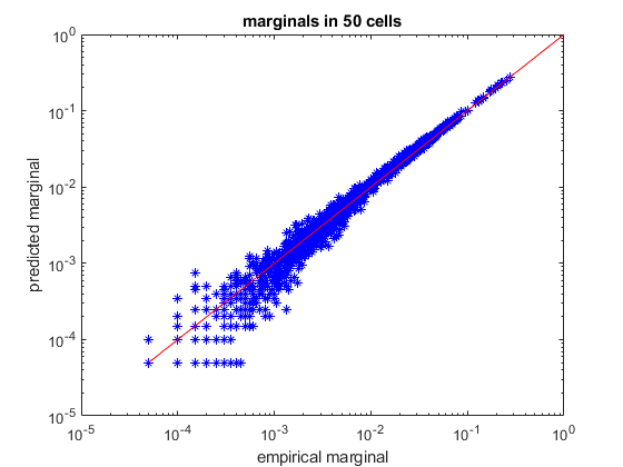
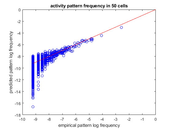
load example50

% randomly divide into train/test sets
[ncells,nsamples] = size(spikes50);
idx_train = randperm(nsamples,ceil(nsamples/2));
idx_test = setdiff(1:nsamples,idx_train);
samples_train = spikes50(:,idx_train);
samples_test = spikes50(:,idx_test);

% create a pairwise maximum entropy model
model = maxent.createModel(50,'pairwise');

% train the model to a threshold of 1.5 standard deviations from the error of computing the marginals.
% because the distribution is larger (50 dimensions) we cannot explicitly iterate over all 5^20 states
% in memory and will use markov chain monte carlo (MCMC) methods to obtain an approximation
model = maxent.trainModel(model,samples_train,'threshold',1.5);


% get the marginals (firing rates and correlations) of the test data and see how they compare to the model predictions.
% here the model marginals could not be computed exactly so they will be estimated using monte-carlo. We specify the
% number of samples we use so that their estimation will have the same amoutn noise as the empirical marginal values
marginals_data = maxent.getEmpiricalMarginals(samples_test,model);
marginals_model = maxent.getMarginals(model,'nsamples',size(samples_test,2));

% plot them on a log scale
figure
loglog(marginals_data,marginals_model,'b*');
hold on;
minval = min([marginals_data(marginals_data>0)]);
plot([minval 1],[minval 1],'-r'); % identity line
xlabel('empirical marginal');
ylabel('predicted marginal');
title(sprintf('marginals in %d cells',ncells));

% the model that the MCMC solver returns is not normalized. If we want to compare the predicted and actual probabilities
% of individual firing patterns, we will need to first normalize the model. We will use the wang-landau algorithm for
% this. We chose parameters which are less strict than the default settings so that we will have a faster runtime.
disp('Normalizing model...');
model = maxent.wangLandau(model,'binsize',0.1,'depth',15);

% the normalization factor was added to the model structure. Now that we have a normalized model, we'll use it to
% predict the frequency of activity patterns. We will start by observing all the patterns that repeated at least twice
% (because a pattern that repeated at least once may grossly overrepresent its probability and is not meaningful in this
% sort of analysis)
limited_empirical_distribution = maxent.getEmpiricalModel(samples_test,'min_count',2);


% get the model predictions for these patterns
model_logprobs = maxent.getLogProbability(model,limited_empirical_distribution.words);

% nplot on a log scale
figure
plot(limited_empirical_distribution.logprobs,model_logprobs,'bo');
hold on;
minval = min(limited_empirical_distribution.logprobs);
plot([minval 0],[minval 0],'-r');  % identity line
xlabel('empirical pattern log frequency');
ylabel('predicted pattern log frequency');
title(sprintf('activity pattern frequency in %d cells',ncells));



% Wang-landau also approximated the model entropy, let's compare it to the entropy of the empirical dataset.
% for this we want to look at the entire set, not just the set limited repeating patterns
empirical_distribution = maxent.getEmpiricalModel(samples_test);

% it will not be surprising to see that the empirical entropy is much lower than the model, this is because the
% distribution is very undersampled
fprintf('Model entropy: %.03f bits, empirical entropy (test set): %.03f bits\n',model.entropy,empirical_distribution.entropy);

% generate samples from the distribution and compute their entropy. This should give a result which is must closer to
% the entropy of the empirical distribution...
samples_simulated = maxent.generateSamples(model,numel(idx_test));
simulated_empirical_distribution = maxent.getEmpiricalModel(samples_simulated);
fprintf('Entropy of simulated data: %.03f bits\n',simulated_empirical_distribution.entropy);

Training to threshold: 1.500 standard deviations
Maximum samples: 17778   maximum MSE: 3.375
361/Inf samples=5466  MSE=6.504 (mean), 57.338 (max) [43]
436/Inf samples=11581  MSE=3.315 (mean), 66.423 (max) [2]
479/Inf samples=17778  MSE=2.391 (mean), 28.954 (max) [2]
514/Inf samples=17778  MSE=1.754 (mean), 22.708 (max) [40]
549/Inf samples=17778  MSE=1.699 (mean), 28.873 (max) [12]
584/Inf samples=17778  MSE=1.642 (mean), 11.995 (max) [45]
618/Inf samples=17778  MSE=1.716 (mean), 11.184 (max) [31]
652/Inf samples=17778  MSE=1.644 (mean), 10.448 (max) [1166]
686/Inf samples=17778  MSE=1.595 (mean), 8.928 (max) [1140]
721/Inf samples=17778  MSE=1.820 (mean), 7.465 (max) [40]
756/Inf samples=17778  MSE=1.508 (mean), 7.806 (max) [12]
791/Inf samples=17778  MSE=1.491 (mean), 9.723 (max) [12]
824/Inf samples=17778  MSE=1.521 (mean), 6.340 (max) [12]
857/Inf samples=17778  MSE=1.412 (mean), 4.215 (max) [675]
891/Inf samples=17778  MSE=1.541 (mean), 6.946 (max) [1264]
925/Inf samples=17778  MSE=1.511 (mean), 5.560 (max) [142]
960/Inf samples=17778  MSE=1.695 (mean), 7.271 (max) [1151]
996/Inf samples=17778  MSE=1.601 (mean), 5.649 (max) [1151]
1031/Inf samples=17778  MSE=1.464 (mean), 4.822 (max) [1151]
1066/Inf samples=17778  MSE=1.291 (mean), 6.976 (max) [410]
1102/Inf samples=17778  MSE=1.331 (mean), 3.873 (max) [23]
1138/Inf samples=17778  MSE=1.297 (mean), 3.436 (max) [258]
converged (marginals match)
Normalizing model...
[...............]
Model entropy: 17.527 bits, empirical entropy (test set): 11.978 bits
Entropy of simulated data: 12.490 bits

part 3: working with RP (random projection) models

% load spiking data of 15 neurons
load example15

% randomly divide it into a training set and a test set (so we can verify how well we trained)
[ncells,nsamples] = size(spikes15);
idx_train = randperm(nsamples,ceil(nsamples/2));
idx_test = setdiff(1:nsamples,idx_train);
samples_train = spikes15(:,idx_train);
samples_test = spikes15(:,idx_test);

% create a random projection model with default settings
model = maxent.createModel(ncells,'rp');

% train the model to a threshold of one standard deviation from the error of computing the marginals.
% because the distribution is relatively small (15 dimensions) we can explicitly represent all 2^15 states
% in memory and train the model in an exhaustive fashion.
model = maxent.trainModel(model,samples_train,'threshold',1);

% now check the kullback-leibler divergence between the model predictions and the pattern counts in the test-set
empirical_distribution = maxent.getEmpiricalModel(samples_test);
model_logprobs = maxent.getLogProbability(model,empirical_distribution.words);
test_dkl = maxent.dkl(empirical_distribution.logprobs,model_logprobs);
fprintf('Kullback-Leibler divergence from test set: %f\n',test_dkl);

% create a random projection model with a specified number of projections and specified average in-degree
model = maxent.createModel(ncells,'rp','nprojections',500,'indegree',4);

% train the model
model = maxent.trainModel(model,samples_train,'threshold',1);

% now check the kullback-leibler divergence between the model predictions and the pattern counts in the test-set
empirical_distribution = maxent.getEmpiricalModel(samples_test);
model_logprobs = maxent.getLogProbability(model,empirical_distribution.words);
test_dkl = maxent.dkl(empirical_distribution.logprobs,model_logprobs);
fprintf('Kullback-Leibler divergence from test set: %f\n',test_dkl);

Training to threshold: 1.000 standard deviations
Maximum MSE: 1.000
64/Inf  MSE=0.088 (mean), 4.981 (max) [65]  DKL: 0.122
134/Inf  MSE=0.014 (mean), 2.213 (max) [65]  DKL: 0.112
converged (marginals match)
Standard deviations from marginals: 0.072 (mean), 0.992 (max) [65]  DKL: 0.110
Kullback-Leibler divergence from test set: 0.125975
Training to threshold: 1.000 standard deviations
Maximum MSE: 1.000
09/Inf  MSE=56.463 (mean), 7086.771 (max) [69]  DKL: 0.243
29/Inf  MSE=0.644 (mean), 58.533 (max) [69]  DKL: 0.121
49/Inf  MSE=0.126 (mean), 15.019 (max) [364]  DKL: 0.108
69/Inf  MSE=0.075 (mean), 8.094 (max) [364]  DKL: 0.103
89/Inf  MSE=0.031 (mean), 3.065 (max) [364]  DKL: 0.100
109/Inf  MSE=0.022 (mean), 3.862 (max) [125]  DKL: 0.097
129/Inf  MSE=0.013 (mean), 2.741 (max) [125]  DKL: 0.095
149/Inf  MSE=0.008 (mean), 1.318 (max) [125]  DKL: 0.094
converged (marginals match)
Standard deviations from marginals: 0.083 (mean), 0.997 (max) [125]  DKL: 0.093
Kullback-Leibler divergence from test set: 0.108484

part 4: specifying a custom list of correlations

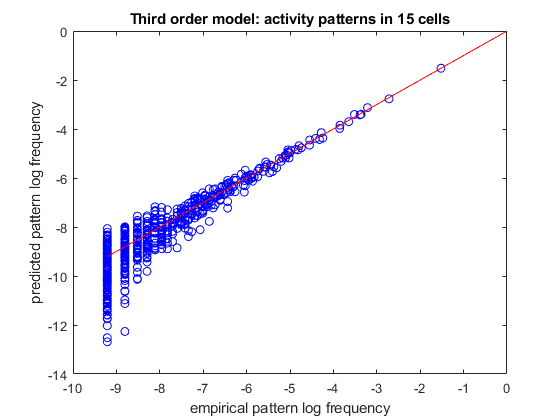
% load spiking data of 15 neurons
load example15

% randomly divide it into a training set and a test set (so we can verify how well we trained)
[ncells,nsamples] = size(spikes15);
idx_train = randperm(nsamples,ceil(nsamples/2));
idx_test = setdiff(1:nsamples,idx_train);
samples_train = spikes15(:,idx_train);
samples_test = spikes15(:,idx_test);


% create a model with first, second, and third-order correlations. (third-order model)
% we will do this by specifying a list of all the possible combinations of single factors, pairs and triplets
correlations = cat(1,num2cell(nchoosek(1:ncells,1),2), ...
                num2cell(nchoosek(1:ncells,2),2),...
                num2cell(nchoosek(1:ncells,3),2));

model = maxent.createModel(ncells,'highorder',correlations);

% train it
model = maxent.trainModel(model,samples_train,'threshold',1);

% use the model to predict the frequency of activity patterns.
% We will start by observing all the patterns that repeated at least twice (because a pattern that repeated at least
% once may grossly overrepresent its probability and is not meaningful in this sort of analysis)
limited_empirical_distribution = maxent.getEmpiricalModel(samples_test,'min_count',2);

% get the model predictions for these patterns
model_logprobs = maxent.getLogProbability(model,limited_empirical_distribution.words);

% nplot on a log scale
figure
plot(limited_empirical_distribution.logprobs,model_logprobs,'bo');
hold on;
minval = min(limited_empirical_distribution.logprobs);
plot([minval 0],[minval 0],'-r');  % identity line
xlabel('empirical pattern log frequency');
ylabel('predicted pattern log frequency');
title(sprintf('Third order model: activity patterns in %d cells',ncells));

Training to threshold: 1.000 standard deviations
Maximum MSE: 1.000
26/Inf  MSE=3.765 (mean), 651.384 (max) [12]  DKL: 0.280
55/Inf  MSE=1.461 (mean), 42.061 (max) [8]  DKL: 0.145
84/Inf  MSE=0.555 (mean), 25.381 (max) [13]  DKL: 0.110
113/Inf  MSE=0.251 (mean), 20.876 (max) [2]  DKL: 0.098
142/Inf  MSE=0.125 (mean), 5.159 (max) [2]  DKL: 0.092
171/Inf  MSE=0.089 (mean), 5.211 (max) [278]  DKL: 0.089
199/Inf  MSE=0.047 (mean), 1.658 (max) [501]  DKL: 0.087
228/Inf  MSE=0.028 (mean), 1.828 (max) [12]  DKL: 0.085
255/Inf  MSE=0.025 (mean), 1.676 (max) [501]  DKL: 0.084
282/Inf  MSE=0.023 (mean), 1.690 (max) [501]  DKL: 0.083
converged (marginals match)
Standard deviations from marginals: 0.116 (mean), 0.990 (max) [501]  DKL: 0.083

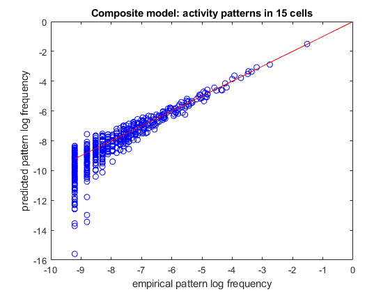
part 5: constructing composite models

% load spiking data of 15 neurons
load example15

% randomly divide it into a training set and a test set (so we can verify how well we trained)
[ncells,nsamples] = size(spikes15);
idx_train = randperm(nsamples,ceil(nsamples/2));
idx_test = setdiff(1:nsamples,idx_train);
samples_train = spikes15(:,idx_train);
samples_test = spikes15(:,idx_test);


% create a model with independent factors, k-synchrony and third-order correlations
% we will do this by initializing 3 separate models and then combining them to a single model
third_order_correlations = num2cell(nchoosek(1:ncells,3),2);
model_indep = maxent.createModel(ncells,'indep');
model_ksync = maxent.createModel(ncells,'ksync');
model_thirdorder = maxent.createModel(ncells,'highorder',third_order_correlations);
model = maxent.createModel(ncells,'composite',{model_indep,model_ksync,model_thirdorder});

% train it
model = maxent.trainModel(model,samples_train,'threshold',1);

% use the model to predict the frequency of activity patterns.
% We will start by observing all the patterns that repeated at least twice (because a pattern that repeated at least
% once may grossly overrepresent its probability and is not meaningful in this sort of analysis)
limited_empirical_distribution = maxent.getEmpiricalModel(samples_test,'min_count',2);

% get the model predictions for these patterns
model_logprobs = maxent.getLogProbability(model,limited_empirical_distribution.words);

% nplot on a log scale
figure
plot(limited_empirical_distribution.logprobs,model_logprobs,'bo');
hold on;
minval = min(limited_empirical_distribution.logprobs);
plot([minval 0],[minval 0],'-r');  % identity line
xlabel('empirical pattern log frequency');
ylabel('predicted pattern log frequency');
title(sprintf('Composite model: activity patterns in %d cells',ncells));

Training to threshold: 1.000 standard deviations
Maximum MSE: 1.000
30/Inf  MSE=0.484 (mean), 26.973 (max) [12]  DKL: 0.122
62/Inf  MSE=0.152 (mean), 4.076 (max) [24]  DKL: 0.111
94/Inf  MSE=0.062 (mean), 2.372 (max) [150]  DKL: 0.106
126/Inf  MSE=0.030 (mean), 1.534 (max) [458]  DKL: 0.104
159/Inf  MSE=0.025 (mean), 4.956 (max) [24]  DKL: 0.103
192/Inf  MSE=0.015 (mean), 1.924 (max) [24]  DKL: 0.101
225/Inf  MSE=0.011 (mean), 1.095 (max) [458]  DKL: 0.100
converged (marginals match)
Standard deviations from marginals: 0.097 (mean), 1.000 (max) [458]  DKL: 0.100

part 6: constructing and sampling from high order Markov chains

train a time-dependent model

% load spiking data of 15 neurons
load example15_spatiotemporal

ncells = size(spikes15_time_dependent,1);
history_length = 2;


% Create joint words of (x_t-2,x_t-1,x_t).
xt = [];
for i = 1:(history_length+1)
   xt = [xt;spikes15_time_dependent(:,i:(end-history_length-1+i))];
end


% create a spatiotemporal model that works on series of binary words: (x_t-2,x_t-1,x_t).
% this essentially describes the probability distribution as a second-order Markov process.
% We will model the distribution with a composite model that uses firing rates, total synchrony in the last 3 time bins
% and pairwise correlations within the current time bin and pairwise correlations between the current activity of a cell
% and the previous time bin.
time_dependent_ncells = ncells*(history_length+1);
inner_model_indep = maxent.createModel(time_dependent_ncells,'indep');  % firing rates
inner_model_ksync = maxent.createModel(time_dependent_ncells,'ksync');  % total synchrony in the population
% add pairwise correlations only within the current time bin
second_order_correlations = num2cell(nchoosek(1:ncells,2),2);
temporal_matrix = reshape(1:time_dependent_ncells,[ncells,history_length+1]);
temporal_interactions = [];
% add pairwise correlations from the current time bin to the previous time step
for i = 1:(history_length)
    temporal_interactions = [temporal_interactions;temporal_matrix(:,[i,i+1])];
end
% bunch of all this together into one probabilistic model
temporal_interactions = num2cell(temporal_interactions,2);
inner_model_pairwise = maxent.createModel(time_dependent_ncells,'highorder',[second_order_correlations;temporal_interactions]);
mspatiotemporal = maxent.createModel(time_dependent_ncells,'composite',{inner_model_indep,inner_model_ksync,inner_model_pairwise});

% train the model on the concatenated words
disp('training spatio-temporal model...');
mspatiotemporal = maxent.trainModel(mspatiotemporal,xt);


% sample from the model by generating each sample according to the history.
% for this we need to generate the 3n-dimensional samples one by one, each time fixing two-thirds of the code word
% corresponding to time t-2 and t-1 and sampling only from time t.
disp('sampling from spatio-temporal model...');
x0 = uint32(xt(:,1));
xspatiotemporal = [];
nsamples = 10000;
for i = 1:nsamples

    % get next sample. we will use burn-in of 100 each step to ensure that we don't introduce time-dependent stuff
    % related to the sampling process itself.
    xnext = maxent.generateSamples(mspatiotemporal,1,'fix_indices',1:(ncells*history_length),'burnin',100,'x0',x0);
    generated_sample = xnext(((ncells*history_length)+1):end,1);

    % shift the "current" state by one time step
    x0 = [x0((ncells+1):end,:);generated_sample];

    % add the current output
    xspatiotemporal = [xspatiotemporal,generated_sample];

end


% plot the result
display_begin = 2000;
nsamples_to_display = 300;


% plot the actual raster
pos = [400,600,700,250];
figure('Position',pos);
subplot(2,1,1);
pos = get(gca, 'Position');pos(1) = 0.055;pos(3) = 0.9;set(gca, 'Position', pos);
imshow(~spikes15_time_dependent(:,display_begin+(1:nsamples_to_display)));
title('Actual data');

% plot raster sampled from a spatiotemporal model
subplot(2,1,2);
pos = get(gca, 'Position');pos(1) = 0.055;pos(3) = 0.9;set(gca, 'Position', pos);
imshow(~xspatiotemporal(:,display_begin+(1:nsamples_to_display)));
title('Synthetic data (2nd-order Markov)');

training spatio-temporal model...
Training to threshold: 1.300 standard deviations
Maximum samples: 47335   maximum MSE: 2.535
283/Inf samples=2488  MSE=19.036 (mean), 47.786 (max) [48]
357/Inf samples=5250  MSE=9.391 (mean), 33.829 (max) [103]
401/Inf samples=8163  MSE=6.096 (mean), 21.037 (max) [212]
431/Inf samples=11016  MSE=4.558 (mean), 17.024 (max) [222]
455/Inf samples=14000  MSE=3.666 (mean), 10.921 (max) [52]
474/Inf samples=16923  MSE=3.058 (mean), 7.152 (max) [59]
490/Inf samples=19851  MSE=2.590 (mean), 7.018 (max) [99]
504/Inf samples=22824  MSE=2.239 (mean), 8.185 (max) [101]
516/Inf samples=25725  MSE=1.969 (mean), 9.438 (max) [101]
527/Inf samples=28707  MSE=1.797 (mean), 8.821 (max) [101]
537/Inf samples=31713  MSE=1.656 (mean), 7.257 (max) [101]
546/Inf samples=34690  MSE=1.598 (mean), 8.343 (max) [212]
554/Inf samples=37567  MSE=1.502 (mean), 8.692 (max) [212]
562/Inf samples=40683  MSE=1.403 (mean), 9.427 (max) [212]
570/Inf samples=44058  MSE=1.310 (mean), 9.120 (max) [212]
577/Inf samples=47239  MSE=1.227 (mean), 8.797 (max) [212]
584/Inf samples=47335  MSE=1.150 (mean), 8.708 (max) [212]
591/Inf samples=47335  MSE=1.082 (mean), 8.041 (max) [212]
598/Inf samples=47335  MSE=1.008 (mean), 7.813 (max) [212]
605/Inf samples=47335  MSE=0.978 (mean), 6.697 (max) [212]
612/Inf samples=47335  MSE=0.925 (mean), 5.669 (max) [212]
619/Inf samples=47335  MSE=0.902 (mean), 5.225 (max) [212]
626/Inf samples=47335  MSE=0.905 (mean), 4.294 (max) [212]
633/Inf samples=47335  MSE=0.908 (mean), 3.184 (max) [212]
converged (marginals match)
sampling from spatio-temporal model...

Published with MATLAB® R2017b